The Weierstrass Approximation Theorem (WAT)
Notes by Betty Mock
Introduction
This theorem is extremely useful, and easy to understand, so it is well worth looking at. The original version of this result was established by Karl Weierstrass in 1885 using the Weierstrass transform. Learn about the transform here. The most common proof used nowadays established in 1912 is via the Bernstein Polynomials.
We will
- state the theorem and some of its extentions
- discuss some uses of the theorem
- describe the Stone-Weierstrass generalizations
- introduce the Bernstein polynomials.
- present Korovkin's theorem significant generalization of WAT
- make the classic Bernstein polynomial proof available to compare to the Korovkin proof
- addendem-- further information
- the classic Bernstein polynomial proof of WAT
- some non-standard proofs and non-proofs
Before we begin
The WAT is about continuous functions, so it seems well to make sure we know what is needed about continuous functions. First, intuitively, a continuous function is one that we can draw without lifting our pencil. See the red curve in the picture below. A discontinuous function will have gaps and jumps in it, so that we can't draw it without lifting our pencil.
Continuous functions are very, very important. There is a wealth of physical phenomena such as gravity and heat transfer whose mathematical descriptions require continuous functions. So if we are to do any physics, we must know about continuous functions. In addition, on top of this essentially simple idea, towers of mathematics have been built, most of them with real world applications.
The intuitive idea is nice, but it is not rigorous. We need rigor because we need to develop a deep understanding of continuous functions, where the ideas may not be intuitive. The rigorous definition currently most used is known as the ε-δ definition, and was first given by Bernard Bolzano in 1817.
To start understanding it, look at the picture below.
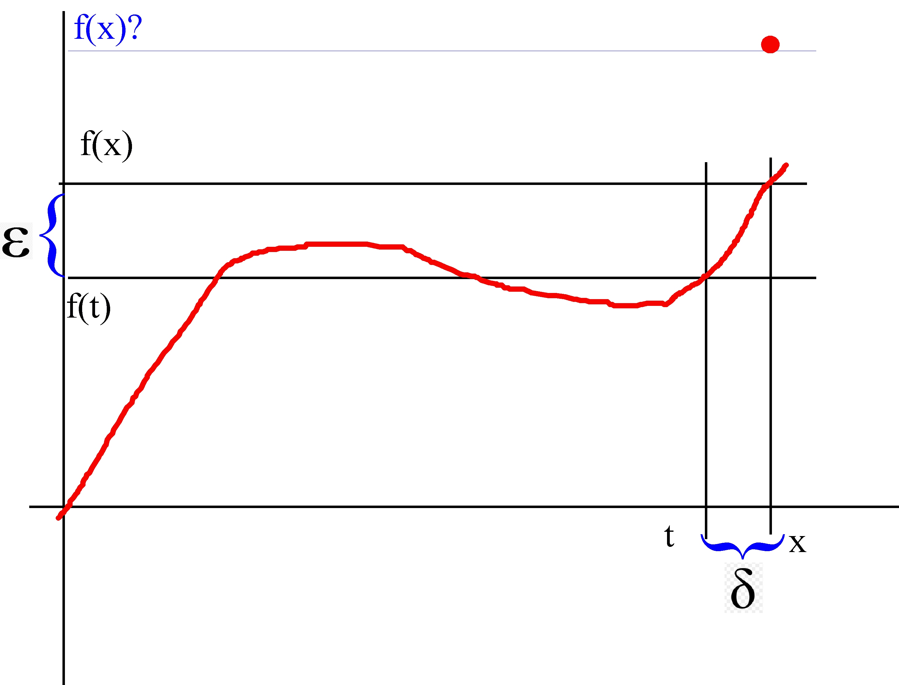
The red curve is f, a continuous function. Now let's suppose we want to state rigorously that f is continuous at x. We begin by considering the difference between f(x) and f(t) (where t is just another point on the x-axis). We call this difference ε. Once we have ε that generates a difference δ on the x-axis -- this is just x-t, or to be perfectly rigorous |x-t|, since t may be to the right or left of x.
Okay, here we go. The function f is continuous at the point x if no matter how small we choose ε we can get |f(t) - f(x)| is < ε if we just get t close enough to x. Rigorously we say it this way:
The function f is continous at x if
(A)
for every ε > 0 there exists a δ such that when |x-t| < δ |f(x) - f(t)| < ε
The operative word in definition (A) is "every". No matter how small an ε you pick, there is a corresponding δ. To make this even a little clearer, pretend that f(x) is not where it has been placed on the red curve, but somewhat above it at the red dot. That leaves a hole in the curve at x. We say, intuitively that f is discontinuous at x. Comparing this situation with the definition (A), we can see graphically that no matter how close t is to x, we'll never get f(t) close to f(x).
Uniform continuity
We're going to need one more concept about continuity before we proceed. This is called "uniform continuity". So far, we've looked at continuity just at one point. A function is continuous on an entire interval (a,b) if it is continuous at every point x in (a,b).
Now a dirty little secret comes out of the woodwork. You'll never see this stated in a calculus book but the fact is that δ depends not just on ε but also on x . The steeper the curve is, the smaller δ has to be to get f(t) sufficient close to f(x). Thus enters the idea of uniform continuity.
The function f is uniformly continuous on an interval if, given an ε there is a δ which is independent of x that works for every point in the entire interval and not just one point. One of the most basic theorems is that if f is continuous on a closed interval [a,b] it is uniformly continuous there. We'll be relying on that to prove the WAT.
Well, what about an open interval? You can't guarantee uniform continuity there, because it's possible for f to become infinitely steep. Just look at the function f(x) = 1/x on (0,1). And that steepness makes uniform continuity impossible.
The Weierstrass Approximation Theorem
If f is a continuous real-valued function on [a,b] and if any ε is given, then there exists a polynomial p (with rational coefficients) on [a,b] such that |f(x) - p(x)| < ε for all x in [a,b].
In other words, any continuous function on a closed, bounded interval can be uniformly approximated on that interval by a polynomial to any degree of accuracy.
This either seems kind of obvious, in which case you likely envision continuous functions as smooth things which are mainly differentiable; or else it seems amazing, if you realize that there are functions on [a,b] which are everywhere continuous and nowhere differentiable. But WAT says even these ugly things can still be approximated by polynomials.
Comment
I love theorems like this, which say that something complicated (K) can be approximated by something simple (S). What that means is there is a standard approach which you can use to prove results about K by bootstrapping your way up from S. Because S is simple it may be easy to prove the result for S. Then you have to show that the result can survive the (supposedly small) jump to K. This works very, very well in all sorts of situations.
Extensions of the Theorem
1. The differentiability approximation
Assume that f has a continuous derivative on [a,b]. Then there exists a polynomial p(x) such that
|f(x) - p(x)| < ε and |f'(x) - p'(x)| < ε
for all x in [a,b]. In other words, you can uniformly approximate both f and f´ with a single polynomial and its derivative. And the same goes for the higher derivatives if they exist and are continuous on [a,b]. The proof is pretty simple. Approximate f'(x) with p'(x) and then take the anti-derivative of p'(x) to get p(x).
2. The Stone-Weierstrass Theorems
Extends WAT in two different directions.
The first is replacing the real interval [0,1] (or [a,b]) with an arbitrary compact Hausdorff space.
Definition
A topological space is said to be compact Hausdorff if
- it is compact (i.e., every open cover has a finite subcover)
- and Hausdorff (i.e., any two distinct points can be separated by disjoint open subsets)
Obviously the real numbers are a Hausdorff space, also the Rn spaces and the complex numbers. This hardly needs illuminating. However, there are other kinds of spaces. One of the simpler is the Hilbert space L2[0,1] (the functions whose squares are Lebesgue integrable [0,1]). There are lots and lots or these spaces and they are important in a great deal of work.
The second is replacing the set of polynomials with other sets of continuous functions, and Stone gives the conditions such a set must fulfill. More information here.
3. The Korovkin Theorems
Korovkin's Theorem #1 is a generalization of the WAT. It will be stated and proved below. It is extremely useful because it takes most of the work out of proving Weierstrass type theorems.
The ideas in Korovkin's Theorem #1 have been expanded on so that there is now a collection of Korovkin type theorems for different kinds of spaces and classes of functions. The approach has been very fruitful. Some of these many theorems turn out to be equivalent to various of the Stone-Weierstrass theorems (not surprisingly). More information (much, much more) here.
Examples of using the WAT
WAT is basically a helper theorem, which makes it easier (or possible) to prove other theorems.
As I commented earlier, having a dense polynomial subset of the continuous functions is enormously useful in proving all sorts of things which might otherwise be resistant or cumbersome. To illustrate we will use WAT to prove some theorems about continuous functions. It would be fun to prove some elementary theorems about continuous functions such as
- A continuous function on a closed interval is bounded there.
- A continuous fucntion on a closed interval is uniformly continuous there
While these theorems are easy to prove using WAT, we can't do it that way, because WAT relies on those theorems for its proof. Going in logical circles is not an approved method of proof (however much easier it makes things). However we can prove these:
- The intermediate value theorem for continuous functions
- Let f be continuous on [0,1] and suppose
- Separable Spaces
x^n.png)
Then f(x) ≡ 0 on [0,1]
Definition
A separable space X is one having a countable dense subset D. Dense means D is a subset of X such that the closure of D = X. That is: the limit of every convergent sequence in D is in X; and every element of X is the limit of some convergent sequence in D.
The real line is a separable space since the rationals are a countable dense subset. What WAT tells us is that the space X(C) of all continuous, real-valued functions on [0,1] is separable. Many spaces of interest are metric spaces whose elements are functions, and the extensions or generalizations of WAT can be used to show that such spaces are separable.
Many, many theorems are true on separable spaces which are not true on non-separable spaces. An example of a non-separable space is described here .
The value of Separability is a generalization of my earlier statement that theorems like WAT are immensely helpful in proofs. We can prove whatever it is for the countable dense subset, and once that is proved jump to the entire set (and hopefully don't plunge to our death on the way).
Compare proofs of 1: intermediate value theorem for continuous functions on a closed interval
The Theorem: If f(x) is continuous on [a,b] and k is strictly between f(a) and f(b), [note f(a) ≠ f(b)] then there exists some c in (a,b) where f(c)=k.
Standard Proof
This proof is from the website here
I find this proof cumbersome, badly written, and not even quite correct. This approach could provide a much clearer (definitely correct) proof. However, sadly it is far too typical of mathematical writing, causing students to think they are not good at math, when it is the writers and presenters who are not good.
Without loss of generality (WLOG) let us assume that f(a) < k < f(b). Define a set S = {x ε [a,b]:f(x)< k} and let c be the sup of S (which exists due to the previous theorem).
Due to continuity at a we can keep f(x) within any ε > 0 of f(x) by keeping x sufficiently close to a. Since f(a)< k is a strict inequality. No value sufficiently close to a can then get greater than k, which means there are values larger than a in S. Hence f(a) cannot be the supremum f(c) = k; some value to its right must be.
Likewise due to the continuity at b we can keep f(x) within some ε > 0 of f(b) by keeping x sufficiently close to b. Since k < f(b) is a strict inequality, Every value sufficiently close to b must then be greater than k, which means f(b) cannot be the supremum c -- some value to its left must be.
Since c ≠ a and c ≠ b, but c is in [a,b] is must be the case that c is in (a,b). Now we hope to show that f(c) = k.
Since f(x) is assumed to be continuous on [a,b] and c ε [a,b] we have limx → c = f(c). Thus for any ε we can find a δ so that whenever c - δ < x < c + δ we must have f(c) - ε < f(x) < f(c) + ε.
Consider any such value ε > 0 and the value of δ that goes with it.
Now that there must exist some x0 ε (c-δ, c) where f(x0) < k. If there wasn't, then c would not have been the supremum of S-- some value to the left of c would be the supremum.
However since c-δ < x0 < c + δ, we also know that f(c) - ε < f(x0)
Focusing on the left side of this string inequality f(c) - ε < f(c) we add ε to both sides to obtain f(c) < f(x0) + ε There also must exist some x1 ε[c, c+δ) where f(x1) ≥ k. If there wasn't the c would not have been the supremum of S -- some value to the right of c would have been. However, since c- δ < x1 < c + δ we also know that f(c) - ε < f(x1) < f(c) + ε (As above the case not inferred by the continuity of f is an obvious one.) Focusing on the right side of this string inequality, f(x1) < f(c) + ε, we subtract ε from both sides to obtain f(x1) - ε < f(c). Remembering that f(x1) ≥ k we have Then combining (1) and (2) we have However the only way this hold for any ε is for f(c) = k. Proof using WAT Restating the theorem: If f(x) is continuous on [a,b] and k is strictly between f(a) and f(b), [note f(a) ≠ f(b)] then there exists some c in (a,b) where f(c)=k. Let us prove that theorem is true for polynomials. Looking at the simplest polynomial p(x) = x (say on [0,1], given a k we can of course simply compute c, but that is no help in moving the general proof forward. Since p(x) = x is monotonic increasing on the entire interval [0,1] and p(a) < k there is an x1 in (0,1) such that a < x1 and p(a) < p(x1) ≤ k.
If the right hand inequality is in fact equal, we are done: c = x1. If not, then because p is monotonic there is an x2 such that x1 < x2 and p(x2) ≤ k. If the ≤ k is really <, we can then go on to x3 and so on constructing a set {xj}. It is not necessary to ever get an equality p(xj) = k. Now choose an ε. Because p is monotonic and continuous, we can choose x2 such that k - ε/2 < p(x2) ≤ k. We can choose x3 > x2 so that k - ε/3 < p(x3) ≤ k; and so on. Since the sequence {p(xn)} is increasing, bounded above by k, and has elements that are arbitrarily close to k, it must converge to k. And since p is continuous in the neighborhood of k then k must be p(something). Might as well call that something c. Notice, we didn't actually use the fact that p(x) = x is linear. The same exact argument can be made for any function which is continuous and monotonic on a closed interval. That thought provides a route to prove the result for any polynomial.
Moving on to the general polynomial p(x) on [a,b], assume WLOG that p(a) < p(b) and p(x) is increasing in the vicinity of a. We note that a polynomial of degree n has as most n-1 inflection points, where p'(x) = 0 in (a,b), i.e. points where there might be a local maximum or minimum. Adding the endpoints a and b there are then at most n+1 points where p takes on a local maximum or minimum. Thus p is monotonic on n intervals within (a,b). Let x1 be the first point where p(x) achieves a local maximum in [a,b]. We have p(a) < (x1) and p is monotonic increasing on (a, x1). Applying the above results there are three possibiities:
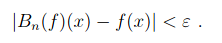
Remember, there are only a finite number of xj that must be considered. At least one of these intervals must have an endpoint which is larger than c, because b is such an endpoint and p(b) > k. Once we find such an endpoint, we have found a subinterval in which p takes on the value k, so we now have a c. We have proved the intermediate value theorem for all polynomials. Going on to a general continuous function, let f be continuous on [a,b] and choose ε. WAT guarantees we can construct a polynomial p1 such that |f - p1| < ε for all x in [a,b]. Given a k such that f(a) < k < f(b), we know there is a point c1 in (a,b) such that p1(c1) = k. So |f(c1 -p(c1)| < ε. Now create a sequence of εj → 0. This generates sequences {pj} and cj such that |f(cj) - pj(c)| < εj which means that |f(cj) - k| < εj. Since εj → 0, then f(cj) → k. By the continuity of f, if f(cj) converges to k, then cj → c as εj → 0. And f(c) = k. Comment The standard proof does not rely on any advanced mathematics. As with all set-theoretic proofs, it is a bit hard to follow, especially if it is presented in a muddled way, as in the sample above. The WAT proof relies on more advanced mathematics --- that is on the specific nature of the derivatives of polynomials. But it is very easy to follow, it shows clearly why the intermediate value theorem must work, and most important, other things can be proved in a similar way. Proof of 3. Nothing to compare because the using WAT seems to be the only way. Restating the problem: Let f be continuous on [0,1] and suppose (3) for every n. Then f(x) ≡ 0 on [0,1] If f is a constant and not zero than (3) will definitely be > 0. So our only choice for a constant is f≡ 0. Suppose p(x) = ax. Then integrating (3) gives us a/(n+2). This is clearly not zero unless a = 0. So if p is a linear polynomial its coefficients must be zero. The same thing applies to p(x) = axk for any k. So (3) is true if f is any polynomial. According to WAT for any ε there is a polynomial p(x) such that |f(x) - p(x)| < ε, throughout [0,1], We have then (4) If (4) is true for every n, then p(x) ≡ 0. And for any ε we can pick a p(x) such that |p(x) - f(x)| < ε. It follows that f(x) ≡ 0. The Bernstein Polynomials In 1912 Bernstein gave a new, constructive proof of the WAT. He described what are now known as the Bernstein polynomials, and showed that if f(x) is continuous they will converge to f(x). This proof is still the standard used in teaching WAT. To my mind it has been superseded by the proof of Korovkin's Theorem, which is both more general and easier to understand. Because the Korovkin theorem is very abstract, we will prove it and then show exactly how it works in the case of the Bernstein polynomials, to show how the abstraction works in a specific case. Consider the expression: (5) where This is of course the binomial theorem. If p + q = 1 then (5) is called a probability distribution. Now set p = x and q = 1-x. This gives us the expression: (6) From here Bernstein found his way to map the continuous functions into the polynomials, like this: (7) (7) is the Bernstein polynomial of degree n associated with f(x). What Bernstein then shows is that if f is continuous on [0,1], Bn[f(x)] converges uniformly to f(x) as n → ∞. The obvious question to ask is: how did Bernstein know that these were polynomials that would converge as desired. I admit that Bernstein must have known much more about all this than I do. However, we can observe that the weights f(k/n) must have been carefully chosen to produce this result. Bernstein's proof is shown later in this document. However the proof of Korovkin's Theorem, while basically following the same playbook is a bit easier to follow. Once Korovkin is established it can be applied to the Bernstein polynomials, and with a bit of manipulation gives the desired result. Korovkin's First Theorem This theorem is quite general, and applies to all sorts of spaces, classes of functions, and classes of potential approximations. For example, our real line interval [0,1] can be replaced with any compact Hausdorff space A (definition in section on Stone-Weierstrass). Our continuous functions f: [0,1] → R can be replaced with any non-empty set D of real (continuous) functions f: A → R. And the approximating functions need not be polynomials. The WAT will drop right out of it, and strangely, the proof is easier than the standard WAT proof via Bernstein polynomials. Definition - Positive Linear Operator Let D be a non-empty set of real functions (in our case the continuous functions) on a compact Hausdorff space A (in our case [0,1]), and L a function of D into D with the following properties: Then L is called a positive, linear operator on D. The linearity requirement will be familiar to you from linear algebra. If f(x) is differentiable then df/dx is a linear operator (but not a positive one). You may not have not previously seen a positive linear operator, but there is nothing deep about it. For example, f(x)→ 2f(x) is a positive linear operator. We will be considering sequences of positive linear operators. Korovkin shows that if these sequences fulfill certain fairly simple properties, they will converge to the original function f. You will note that f(x)→ af(x) is not going to fulfill those requirements (unless a is 1 or 0, which is not helpful). Korovkin's Theorem 1 Let A = [0,1] and let {Ln} n = 1,2,.. be a sequence of positive linear operators on D such that where an, bn, cn → 0 uniformly on A as n → ∞ Then for any f ε D which is continuous on A, Ln[f(x)] → f(x) uniformly on A as n → ∞ When you look at the proof of WAT using Bernstein polynomials, written out in the addendum, you will notice that they are very similar. This certainly is not accidental. Korovkin obviously noticed that the Bernstein polynomial proof will generalize quite nicely to any positive linear operators. Proof For any ε > 0 there exists a δ such that |f(t) - f(x)| < ε whenever |t - x| < δ If |t-x|≥ δ then (8) |f(t) - f(x)| ≤ 2sup║f║(t-x)2|/δ2 (8) is from the triangle inequality, and relies on |t-x|≥ δ. Thus |Ln εLn (9) ε(1 + αn(x)) + 2║f║/δ2 * {γn(x) + 2x βn(x) +x2αn(x)} We are nearly done here. Looking at (9) we have the following information: Condensing the steps leading to (9) we get that for any chosen ε there is an N such that n > N ⇒ |Ln So |Ln Applying Korovkin to the Bernstein Polynomials What we have to show is that Bn[f(x)] is a positive linear operator on [0,1] and that they satisfy the conditions a, b, and c above. From (7) we see that Bn[f(x)]is a linear operator and must be positive on [0,1] where f is positive. a. Substitute p = x and q = (1-x) into (5). We have that p + q = 1, so for f(x) = 1 we have Bn[1] = 1 b. c. We start with the formula (11) This formula is used in giving a direct proof that the Bernstein Polynomials for f(x) do converge to f(x). The proof of this is I'm going to work now not straightforward, despite the numerous websites which claim it is simple to derive from various formulas, or from the binomial theorem directly. All but one of these sites declined to actually present a proof. The one that did came up with something so cumbersome it was very hard to follow. You will find two proofs here:
here Neither of these proofs show that this is a simple consequence of the previous identities and/or the binomial theorem.
From (11) you can derive If f(x) = x2 then Bn[f(x)] = x2 + x(1-x)/n You do this by expanding the expression (k/n-x)2, then split the left side of (11) 3 sums. The first of these is Bn[x2]. The second two will add up to -p2. Combining that with (11) gives you the result. So the mapping f(x) → Bn[f(x)] is a positive linear operator on [0,1] which satisfies a, b, and c. Korovkin's theorem says Bn[f(x)] must converge to f(x) as n → ∞.
************************************************ Addendum Direct proof of WAT using Bernstein Polynomials Define (12) We will show that for any ε >0 there exists N such that for all n > N and all x in [0,1] Since [0,1] is compact, if f is continuous there, it is uniformly continuous as well. So given ε > 0 there exists a ≤ > 0 such that (13) |x - y | ≤ δ ⇒ |f(x) - f(y)| ≤ ε/2 for all x,y in [0,1] Using (12 we can write where (x,n) is the binomial coefficient. And because the Bernstein polynomials are non-negative on [0,1]
(14) The first term of (14) is easy -- it is less than ε/2 as per (13). For the 2nd term we lean on the condition |k/n -x| ≥ δ and play some arithmetic tricks. Some other attempts to prove WAT. The following two proofs of WAT were offered on the Math Stack Exchange 1. Using Interpolation This attempted proof has a serious flaw. Can you find it? Since f(x) is continuous on [a,b] it is uniformly continuous This means that for any ε > 0 there exists a positive number δ such that |f(x) - f(y)| < ε whenever |x-y| < δ. Let's choose a finite set of points x1,x2...xn in [a,b] such that the intervals (xi-δ,xi+δ for i = 1,2,...,n cover [a,b]. We can do this by dividing [a,b] into subintervals of length 2δ and choosing one xi from each subinterval. Next we will use these points to construct a polynomial p(x) that approximates f(x). We use the Lagrange Interplating Polynomial, which is a polynomial of degree at most n-1 that passes through the n points given by where li(x) is the i-th Lagrange basis polynomial, defined as: By construction p(x) passes through the points (xi, f(xi)) so
|f(xi) - p(xi)| = 0 for all i By the triangle inequality, Since f(x) is uniformly contnuous on [a,b] and each li(x) is continuous on [a,b], it follows that |f(x) - p(x)|< ε for all x in [a,b] 2. Using Fourier Expansion with Fejer theorem Let f: [0,1] → R be continuous. Extend f to be continuous f: [0,2π] with f(0) = f(2π). Let Σj ≥ 0(Ajcosjx+Bjsinjx) be the Fourier series for f. Let
Comment This looks okay to me. Using Fourier series is an alternate approach which is not much in use. The proof is constructive, although not very usefully so. It may be limited in how much it can be generalized.
f(c)< k+ε (1)
k-ε< f(c) (2)
k-ε < f(c) < k + ε
1
∫
(|p(x) - f(x) |xn dx < ε ∫ xn dx = ε/(n+1)
0
1
∫ |p(x) - f(x) |xn dx = | ∫p(x)xndx - ∫f(x)xndx | =
0
∫| p(x) xn dx| ≤ ε/(n+1)
n
Σ 
pkqn-k
= (p + q)n
k=0
n
pn(x) = Σ xk(1-x)n-k
k=0
n
Bn[f(x)] = Σ f(k/n) xk(1-x)n-k
k=0
Ln
+ sup|f(t) - (f(x)|>
|t-x| < δ |t-x|≥ δ
I'm going to work now

2.png)
n
Bnf(x) - f(x) = Σ
[f(k/n)- f(x)]) (x,n)xk(1-x)n-k
k = 0
|Bnf(x) - f(x)| = Σ
[f(k/n)- f(x)]) (x,n)xk(1-x)n-k + Σ [f(k/n)- f(x)]) (x,n)xk(1-x)n-k
|k/n -x|<δ > |k/n -x|≥δ

n
p(x) = Σ
f(xi) li(x)
i=1
n
li(x) = Π
(x-xj/(xi-xj)
j=1
n
|f(x) - p(x)| ≤ Σ
|f(x) - f(xi)|| li(x)|
i=1
n
|fn(x)| = Σ Ajcosjx+Bjsinjx
j=0
Fejer's Theorem says that gm → f uniformly as m → ∞ Now each term in any gm can be uniformly approximated on [1,2] by a finite portion of its power series, giving the Weierstrass Theorem for f: [0,1] → R .
m
Let gm(x) = (1/m+1) Σ fn(x)
j=0